Create Atomic Metrics

Concept

Atomic metrics are indivisible metrics in business definitions and are the most basic metrics. Subsequent composite and derived metrics can be created based on atomic metrics. Atomic metrics are usually measures under a specific business event behavior, used to quantify and statistics the performance of products or businesses. The method is usually aggregation calculation, for example, Net Profit = sum(Order Net Profit), Total Transactions = count(distinct Order No).

Operation Steps

1. Select "Metric Center > Metric Topic" in the navigation bar, click the "New Metric" button, and select "Atomic Metric".

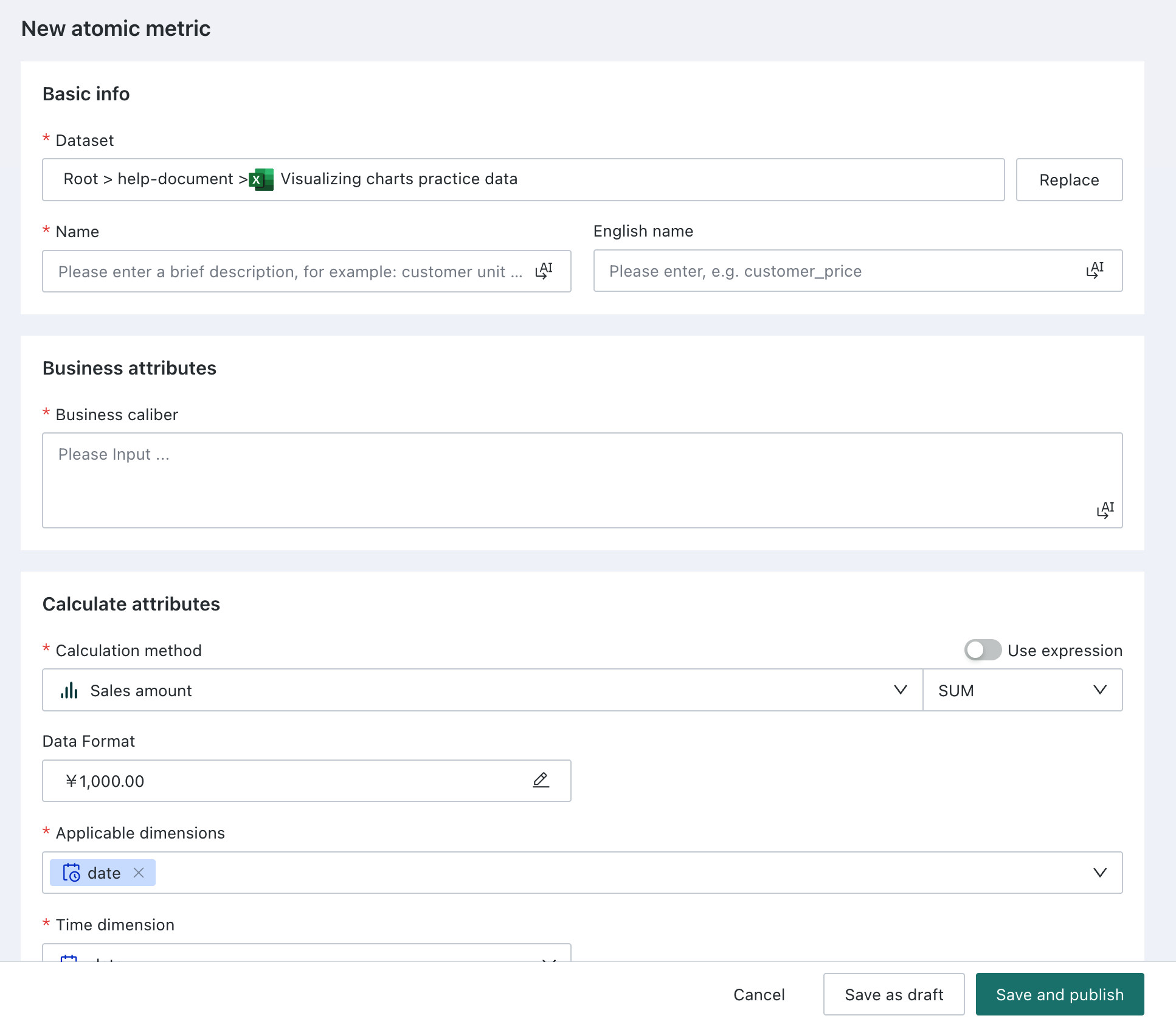
2. In the "New Atomic Metric" dialog, set the basic properties, calculation properties, and management properties of the atomic metric.

   

• Basic Properties

Parameter	Description
Dataset	Select a dataset with usage permissions and use the content of that dataset to create the metric.
Name	Set the Chinese name of the metric, which cannot be repeated under one topic.
English Name	Set the English name of the metric, which cannot be repeated under one topic.

• Calculation Properties

** Parameter**	Description
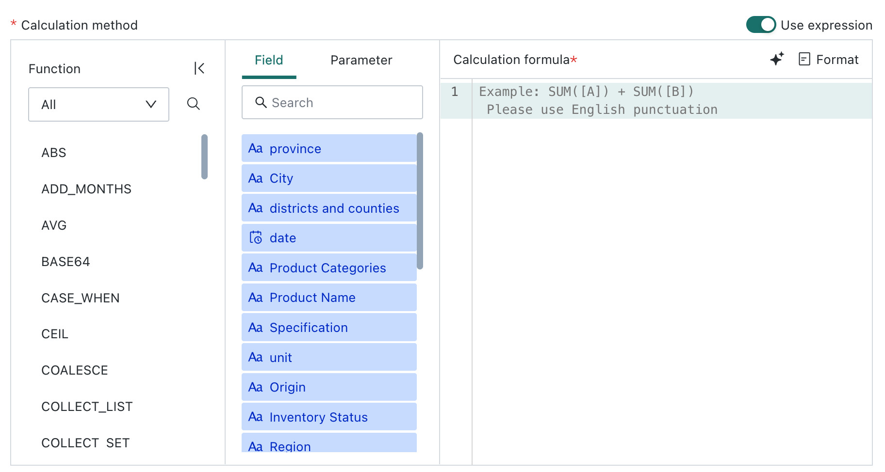
Calculation Method	Source Field: Select a field in the dataset as the source field for calculating the metric's measure value. Aggregation Method: Set the aggregation logic for that field, such as sum, min, max, etc. Use Expression: Use a custom expression to define the aggregation result of the metric, which can reference fields of the currently selected dataset for detailed calculations first. Note: The outermost layer of the expression must be an aggregation function.
Data Format	Set the display format of the metric result.
Applicable Dimensions	Select fields from the dataset as dimensions, which can be used for metric analysis under different dimensions later. When there is a time field in the applicable dimensions, it can be selected as a time dimension for subsequent time-related derivation configuration.
Filter Condition	Supports adding multiple filter conditions. When calculating the metric value, the final result will be calculated according to the filter conditions.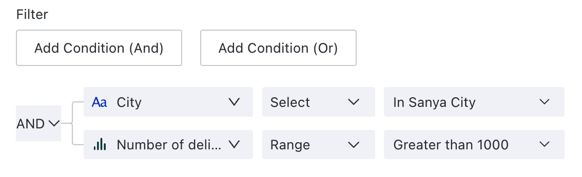
Business Caliber	Maintain the business meaning of the metric to facilitate subsequent metric applications.

• Management Properties

Parameter	Description
Save Location	Set the save location of the metric.
Owner	The interpreter of the business caliber, responsible for the rationality and accuracy of the business caliber.

• Global Parameters

  Atomic metric expressions support the use of global parameters. When metrics are analyzed in dashboards, filters can be linked to parameters of metric cards

  • Supports configuring default values for global parameters on metrics. If not configured, the global parameter default values will be inherited.
  • Parameter effective priority: Filter value > Metric default value > Global parameter default value
  • Special scenario: If there are 2 metrics A and B on a card, both referencing the same global parameter c, with default values c1 and c2 respectively on the metrics. If the filter configures a default value c3 for c, the values of global parameter c for both metric A and metric B will be changed to c3.

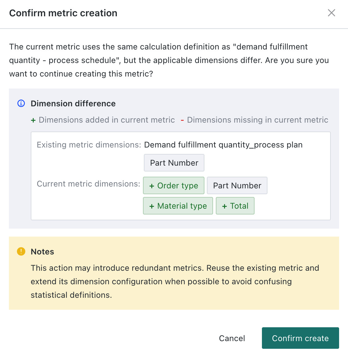
1. After filling in, click "Save and Go Live". If the new metric has the same caliber as an existing metric, the system will verify whether their applicable dimension ranges are consistent and prompt that there is a metric with the same caliber.

   

Query Acceleration

The atomic metric detail page adds configuration query acceleration, supporting configuration of multiple groups of source datasets, source fields, and aggregation methods (only sum and count are supported). It also supports priority sorting. When querying metric data, it will prioritize querying from the dataset with the highest priority.

In principle, metrics are created on detail tables, with sufficient applicable dimensions configured. The associated query acceleration tables are summary tables/dimension reduction tables for that table.

Example: Atomic metric sum (Sales Amount), the source dataset when defining the metric is Table 1, with dimensions Province, City, District, Store. Associated tables are Table 2 and Table 3. Priority is set to Table 3 > Table 2 > Table 1.

Table 1

Province	City	District	Store	Sales Amount
A	A	A	a	1
A	A	A	b	2
B	B	B	c	3
C	C	C	d	4
C	D	D	f	5

Table 2

Province	City	District	Sales Amount
A	A	A	1+2
B	B	B	3
C	C	C	4
C	D	D	5

Table 3

Province	Sales Amount
A	1+2
B	3
C	4+5

• If both the dimension and filter fields exist in Table 3, query from Table 3;
• If the applicable dimension does not exist in Table 3, check whether it exists in Table 2 and query from Table 2;
• If the applicable dimension does not exist in both Table 3 and Table 2, query directly from Table 1.

Examples

(1) Inventory Market Value

Calculation logic: Within the statistical date, the inventory market value of each store = Product Tag Price * Inventory Quantity

Table structure: Date, Store, Category, SKC, Price, Inventory Quantity

• Calculation caliber:

sum(Price * Inventory Quantity)

• Applicable dimensions: Store, Category, Date

(2) On-hand SKU Count

Calculation logic: Count the number of product SKUs with inventory in the store

Table structure: Date, Store, SKC, On-hand Inventory Quantity

• Calculation caliber:

count(distinct concat(`Store`, '_', `SKC`)

• Applicable dimensions: Date, Store
• Filter: On-hand Inventory Quantity > 0

(3) R&D Person-Days Statistics

Calculation logic: R&D person-days = Total Work Hours / Standard Work Hours. Before 2025, the standard work hours per day is 7 hours; after 2025, it is 8 hours per day. Average person-days within the statistical date.

Table structure: Date, Total Work Hours

• Calculation caliber:

SUM(CASE
 WHEN ([Date] < '2025-01-01') THEN ([Total Work Hours])/7
 ELSE [Total Work Hours]/8
END
)

• Applicable dimensions: Date