Create a Historical Zipper Table with Time-Series UDFs

Are you still struggling with where to store historical snapshot data that easily reaches billions or even tens of billions of rows? Are you still frustrated by painfully slow queries on historical snapshot data? Guandata provides a BI solution for historical zipper tables to help solve these problems.

The term "historical zipper table" was not invented by Guandata. After years of practice and refinement by data warehouse builders, historical zipper tables have long been used for compressed storage and querying of massive historical data. However, building and maintaining zipper tables in relational databases usually requires multiple complex steps, such as zipper initialization, opening chains, closing chains, and incremental updates. Each step requires users to clearly understand zipper table operation logic and be proficient in SQL. Therefore, this method is usually difficult to master unless you are an experienced data warehouse engineer, let alone design zipper tables directly in a BI analysis platform.

With the Spark computing engine, the Guandata data analysis platform greatly simplifies the construction and maintenance process of historical zipper tables. It provides a set of custom functions for building and querying historical zipper tables (time-series UDFs), allowing users to build historical zipper tables with only a few functions and support efficient queries.

Introduction to Historical Zipper Tables

During data warehouse construction, we often encounter large-scale data problems with the following characteristics:

1. The overall data volume is large, such as store + SKU-level inventory information.
2. Some fields in the table are continuously updated over time, but the data updated each day is only a small part of all data. In the preceding example, store + SKU combinations with sales movement may account for only 10% or even less of all combinations.
3. Users need to view historical snapshot information at any point in time.

The most direct solution is to store full snapshot data for every day, provide a date primary key, and let users query it. However, this stores a lot of unchanged information and wastes storage. In addition, poor design can seriously affect query efficiency and overload the database.

For example, a chain pharmacy company has 3,000 stores and 1,000 SKUs. If inventory snapshot data is stored, each day contains 3 million rows, and one year contains 1 billion rows. If five years of historical data must be queryable, nearly 5 billion rows of historical snapshot data need to be stored.

Historical zipper tables were created to solve this problem. A historical zipper table maintains both historical status and latest status data. The data stored in a zipper table is essentially equivalent to snapshots, but optimized by removing some unchanged records. With a zipper table, customer records at a zipper point can be easily restored. A zipper table can satisfy the need to reflect historical data status while maximizing storage savings and improving query efficiency. Next, let's look at how the Guandata data analysis platform helps you quickly build historical zipper tables and query snapshots.

Build an Inventory Zipper Table

Prerequisites

1. You need a historical inventory snapshot table. It usually contains date, basic product information, and inventory data, such as inventory amount. If you need to create a snapshot table in BI, see Create Data Snapshots with ETL. If the source data is inbound and outbound inventory details (inventory transaction records), you can skip the data snapshot step and build the inventory zipper table from the daily summarized inventory transaction table.
2. You need to use Guandata zipper table custom functions. The latest list of time-series UDFs is as follows.

Type	Function	Parameter	Output Data Type	Description
Build query table fields (for ETL)	date_range_build_v2	(struct_array)	dateRangStruct	Uncompressed time-series values. The `struct_array` array in the parameter needs to be aggregated by functions such as `collect_list(struct(date, value))`.
	date_text_range_build_v2	(struct_array)	dateTextRangStruct
	date_range_zipper	(dateRangStruct)	dateRangStruct	Time-series values compressed by adjacent equal values. It adds a record with value null for missing dates and compresses it. If a missing date exists and the previous date's value is not null, it adds a record adjacent to the previous date with value null, then compares the current date with the newly added record for compression. It also deduplicates adjacent records with equal values and keeps only the first one.
	date_text_range_zipper	(dateTextRangStruct)	dateTextRangStruct
	date_range_merge	(dateRangStruct_1, dateRangStruct_2)	dateRangStruct	Merges time series without compressing adjacent equal values after merging.
	date_text_range_merge	(dateTextRangStruct_1, dateTextRangStruct_2)	dateTextRangStruct
	date_range_period_to_date	(dateRangStruct, period:string)	dateRangStruct	period: 'week','month','year'. 1. Keeps original dates and accumulates values by the specified period. 2. Fills the start date of missing periods and fills values with 0. It also compresses adjacent equal values after filling and keeps only the first one. This is suitable for calculating and looking up cumulative values within a period, such as weekly, monthly, or yearly cumulative sales.
Look up data (for cards)	date_range_lookup	(dateRangStruct, lookup_date)	Number value	Rolls upward to find the nearest previous date when no data exists for the corresponding date. Suitable for inventory data or member status lookup.
	date_text_range_lookup	(dateTextRangStruct, lookup_date)	String value
	date_range_get	(dateRangStruct, lookup_date)	Number value	Exact lookup. Suitable for sales data lookup. Returns null if no value is found.
	date_text_range_get	(dateTextRangStruct, lookup_date)	String value

1. Function usage notes
2. A date-format field is required in the dataset as the primary key. If a datetime (timestamp) field is used, hour, minute, and second information is not retained.
   1. Functions with text in the name are used to process date primary keys and text fields. Other functions are used to process date primary keys and numeric fields.
   2. Among the preceding functions, date_range_build_v2 and date_text_range_build_v2 first process the original date primary key date and the result field value to be queried (numeric or text field) into a struct_array array. It needs to be aggregated by functions such as collect_list(struct(date, value)).
   3. The struct function merges two columns into one column where field names and field values correspond one to one (key-value pairs). It also converts dates to the computer default Unix date. The start time 1970-01-01 is converted to numeric value 0, and later dates increment by day.
   4. The collect_list function merges multiple rows into one row by group. After conversion, the result is an array format. It must be used together with group by or a window function such as over(partition by ).
   5. The date_range_build_v2 and date_text_range_build_v2 functions reorganize the resulting struct_array and produce a key-value pair. k is an ascending date array, and v is the corresponding inventory count array.
3. The step-by-step processing results and formats are shown below:

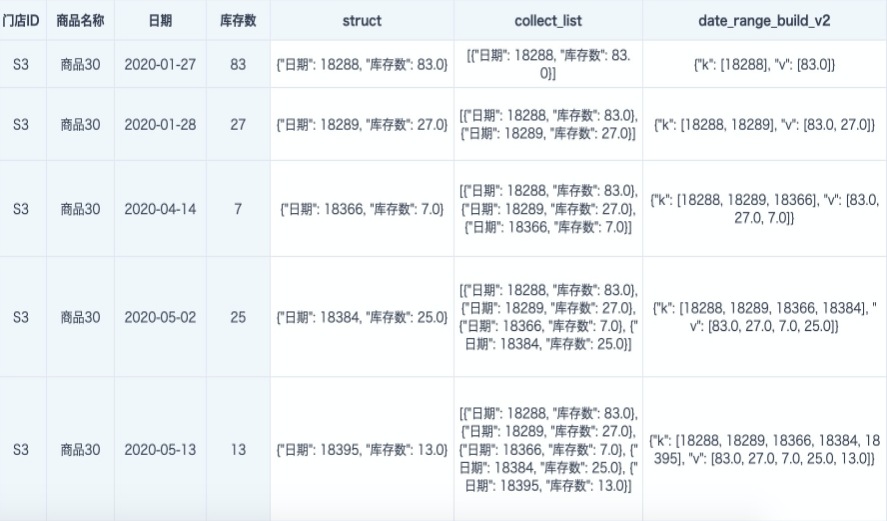
1. The dateRangStruct/dateTextRangStruct produced by date_range_build_v2 and date_text_range_build_v2 can continue to use other time-series UDFs for compression, merging, period-based accumulation, or querying.
2. The legacy functions date_range_build(date_array, value_array) and date_text_range_build(date_array, text_array) can still be used, but only in scenarios where the date and value fields contain no null values. If null values exist, they need to be replaced in advance. Because collect_list discards null values, if the date or numeric value contains null, the correspondence will be misaligned and some data will be lost. For example, if a numeric value is null, its corresponding date will be matched to the next date's value, and the last date will be discarded. Therefore, date_range_build_v2(dateRangStruct) and date_text_range_build_v2 now replace the legacy functions. Similarly, the original date_range_remove_adjacent_same_values(dateRangStruct) and date_text_range_remove_adjacent_same_values(dateTextRangeStruct) are now replaced by date_range_zipper(dateRangStruct) and date_text_range_zipper(dateTextRangStruct). In general, we recommend using the new functions.

Implementation Steps: Inventory Snapshot Table Example

1. Import the prepared snapshot table into the Guandata data platform, create a Smart ETL, and first aggregate the data to the required granularity.

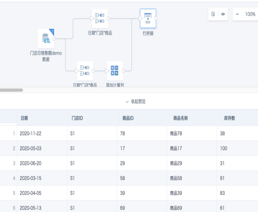
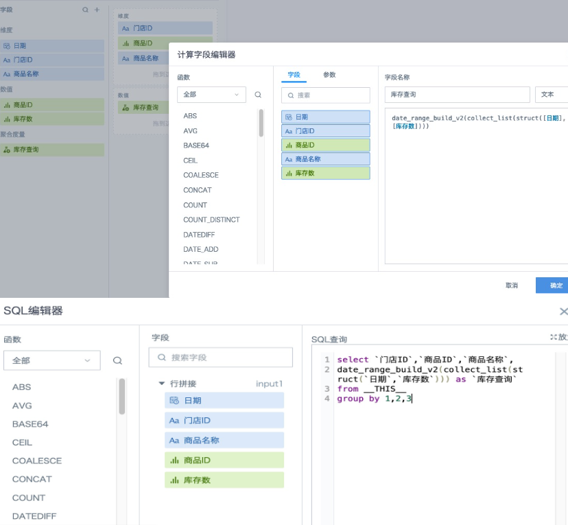
1. Add a group aggregation node and add an aggregate field named "Inventory Lookup". Set the field type to "Text". Then drag the required dimension fields to the dimension area and the aggregate field "Inventory Lookup" to the measure area for group aggregation calculation. The field expression is:

-- Method 1: Recommended
date_range_build_v2(collect_list(struct([Date],[Inventory Count])))
-- Method 2: If you are more used to processing data with SQL, you can also use an "SQL Input" node. The SQL expression is:
select `Store ID`,`Product ID`,`Product Name`,
date_range_build_v2(collect_list(struct(`Date`,`Inventory Count`))) as `Inventory Lookup`
from __THIS__
group by 1,2,3
-- Method 3: You can also create multiple new fields (all with field type "Text").
-- Use struct(), collect_list() over(partition by ), and date_range_build_v2() step by step to obtain calculation results, and then use a group aggregation node to aggregate the data.

At this point, an inventory zipper field is obtained, and the snapshot data has already been greatly compressed.

1. Next, for inventory data, some products may not have inventory changes for a long time. This means there may be many consecutive duplicate values in the inventory count array above. Therefore, add a calculated column and use the date_range_zipper function to further compress the inventory snapshot key-value pairs and build the inventory zipper field. The compression method is as follows: add a record with value null for missing dates and compress it. If a missing date exists and the previous date's value is not null, add a record adjacent to the previous record with value null, then compare whether the current date should be compressed with the newly added record. At the same time, deduplicate adjacent records with equal values and keep only the first one. In short, it has two effects: removing duplicate data and filling missing time periods with null.
   Based on these two effects, when creating a zipper table from a snapshot table, we recommend using date_range_zipper for deduplication. When creating a zipper table from a transaction table, you do not need to, and should not, use date_range_zipper for deduplication.
   After using date_range_zipper([Inventory Lookup]), the data compression result is as follows:

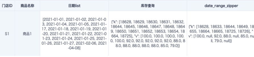
Figure explanation:

From 2021-01-01 to 2021-01-05, the inventory count is always 100. After 5 records are compressed, only one record remains: 2021-01-01 (18628, 100). Data from 2021-01-06 to 2021-01-16 is missing, so dates are automatically filled, inventory count is filled with null, and the result is compressed into one record: 2021-01-06 (18633, null). The same logic continues until completion.

1. If you need to calculate monthly-to-date (MTD) statistics for inventory count, add a calculated column named "MTD Inventory Lookup".

-- In addition to monthly accumulation, yearly ('year') and weekly ('week') accumulation are also supported.
[MTD Inventory Lookup]:date_range_period_to_date([Inventory Lookup],'month')

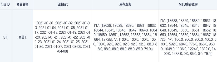
Figure explanation:

Data exists in January, February, and April 2021, and inventory counts are accumulated by month. For example, the final cumulative value for January is 1488. Starting from February, the first day of each month is automatically filled as the period start date. 2021-02-01 corresponds to 18659 and inventory count is filled with 0. 2021-03-01 corresponds to 18687 and inventory count is 0. For April, the period start date and inventory count are also automatically filled. However, because March has no other valid data and the 2021-03-01 data (18687, 0) is an adjacent equal-value record, the 2021-04-01 record is compressed and deduplicated.

Note:

The date_range_period_to_date function can only accumulate inventory numeric values after date_range_build_v2. It cannot process text data in date_text_range_build_v2, nor can it calculate data compressed by date_range_zipper because the filled null values cannot participate in calculations and deduplicated data is not suitable for accumulation.

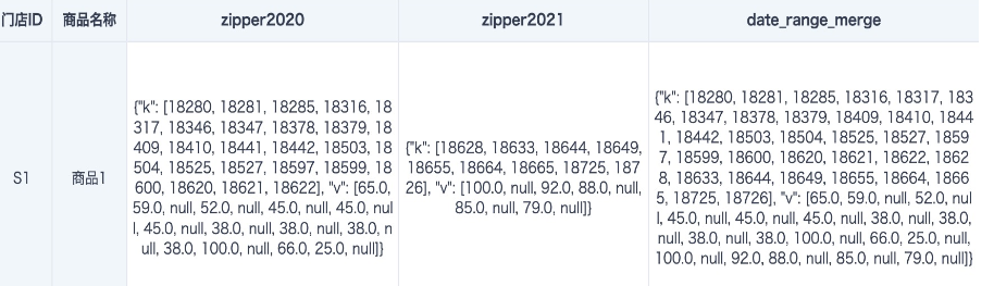
1. If you have inventory zipper tables for two different years and want to merge them to support cross-year queries, first join the two inventory zipper tables by primary key, and then use the date_range_merge() function to merge the two inventory zipper fields without compression.

date_range_merge([zipper2020], [zipper2021])

1. Add an output dataset to the ETL, save and run it, and obtain a historical inventory zipper table with greatly reduced data volume.

Query the Inventory Zipper Table

After the historical inventory zipper table is built, how do you query inventory count for any date on a dashboard? Because the table no longer has an independent date field, you need to use date_range_lookup or date_range_get together with a global parameter to query data.

Implementation Steps

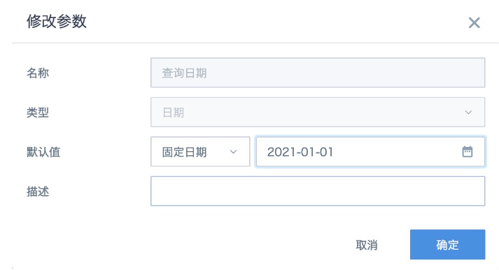
1. Create a date-type global parameter, or use an existing date-type global parameter in the system.

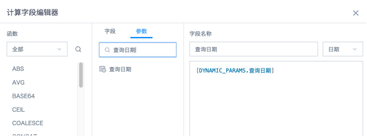
1. Create a card, add a calculated field, directly click the date parameter "Query Date" in the parameter list on the left to reference it, set the field type to "Date", and then drag it into the dimension area.

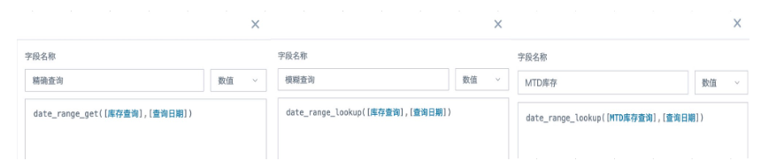
1. Create calculated fields named "Exact Query", "Fuzzy Query", and "MTD Query" as needed. Set the field type to "Numeric", then drag them into the measure area and set the aggregation method to "No Processing".

1. Save the card and return to the page. Create a date-type filter. When linking the card, select the global parameter "Query Date" used by the card and save. Alternatively, create a parameter filter, reference the global parameter "Query Date", and save. The parameter filter automatically links cards on the current page that use the same global parameter. Use normal selection filters to link other dimension fields. The query result is shown below.

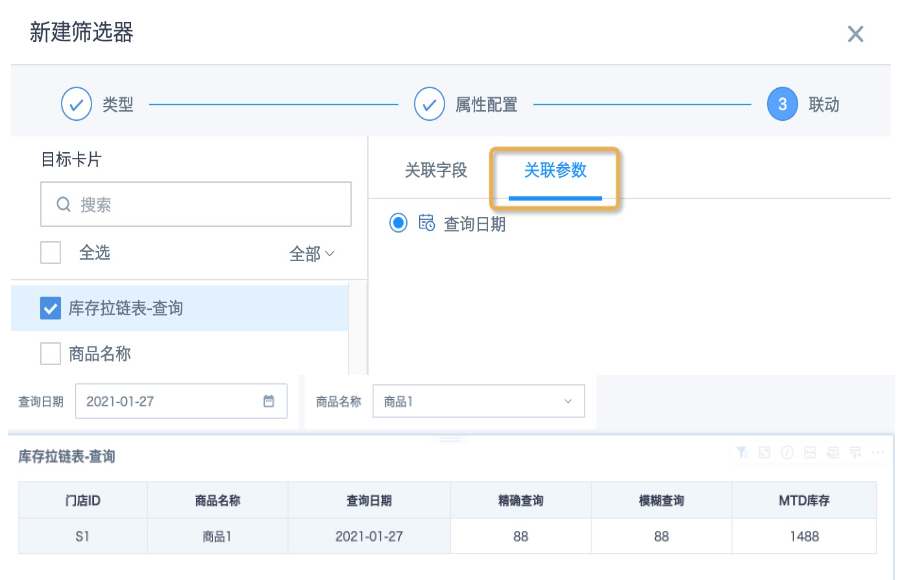
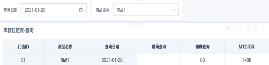
Figure explanation:

Data exists on 2021-01-27, so both exact query and fuzzy query can find the corresponding inventory count 88, and MTD inventory is 1488. No data exists on 2021-01-28, so exact query returns no result, while upward rolling lookup returns the inventory count 88 and MTD inventory 1488 from 2021-01-27.