Build a Simple Monthly Sales Report
Overview
This article demonstrates how to create a single-view monthly sales report from scratch. A single-view report means data preparation is completed from one dataset, or one data source, to generate one view and build one report.
For the video walkthrough of this case, see Chinese-style Reporting Pro - Basic Example Demo 1.
Example Description
The dataset used in this example is: Chinese-style Reporting Pro - Basic Dataset 1.
The table structure of the data source is shown below:
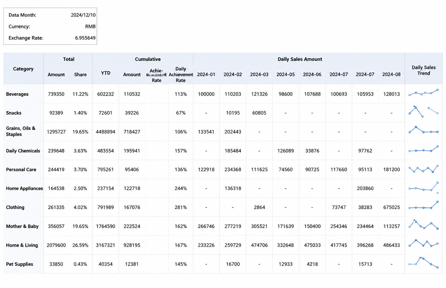
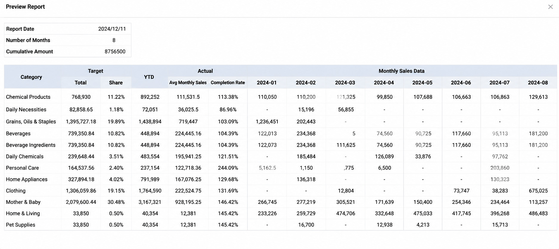
The final result is shown below: Category expands vertically; target values such as Total and Percentage, actual values such as YTD, Average Monthly Sales, and Target Completion Rate, plus monthly sales data, all expand vertically by category; a monthly sales trend sparkline is also displayed and expands vertically by category; the report date, number of months, and cumulative amount are calculated by formulas.
Implementation Idea
- Build the table framework in the worksheet using a static header made of multiple static text cells. In this example, the static header is created by importing an Excel template.
- Based on the static header, drag dimension fields into the sheet and expand them horizontally or vertically as needed, turning the header into a dynamic header that prepares the report for later data filling.
- Drag the measure fields into cells and configure parent cells to support aggregated calculation and dynamic expansion.
The Target Percentage field must be calculated. The target percentage of a category equals the category's total target divided by
SUM(all category target totals). This calculation can be created by Advanced Calculation. For details, see Data Preparation. - Use the insert feature to add sparklines, then configure parent cells so the monthly trend chart expands vertically by category.
- Use Excel functions to calculate the report date, the number of months, and the cumulative amount.
Step-by-Step Example
Data Preparation
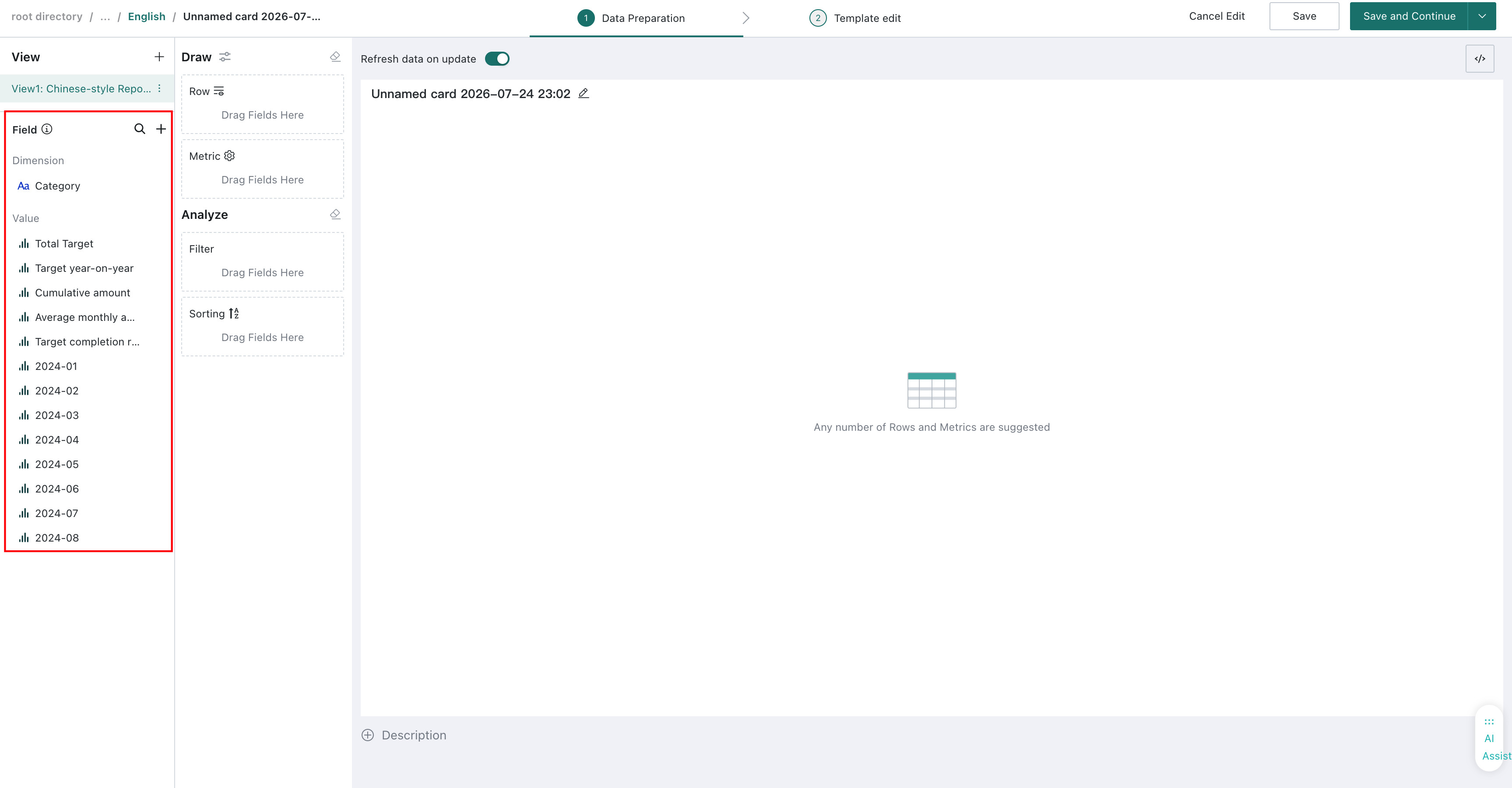
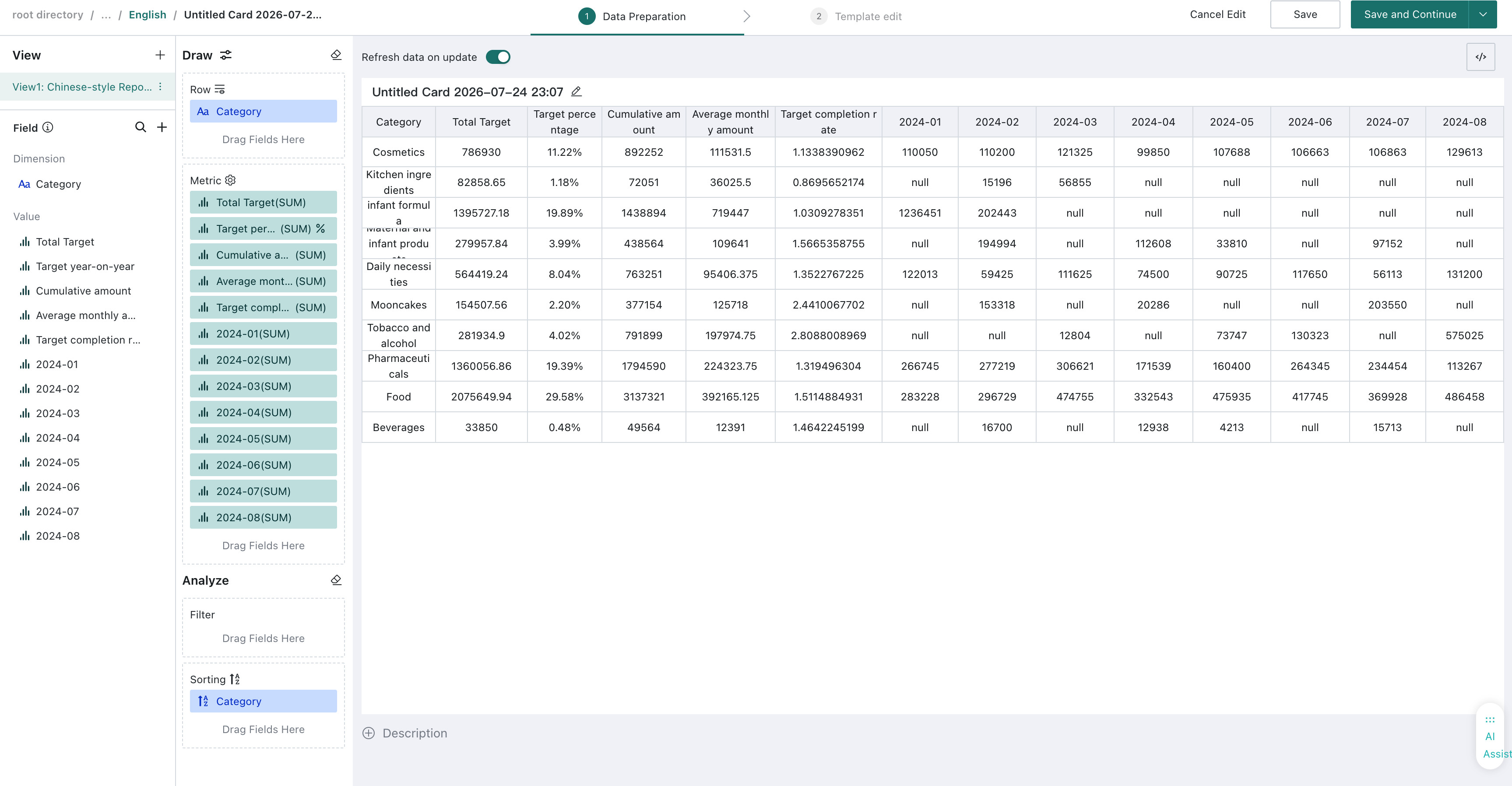
Create a new Chinese-style Reporting Pro card and select the dataset for this example. The raw data in this case is already well prepared, so only Target Percentage needs to be calculated. Configure the charting area as follows:
-
Drag the required fields into the corresponding areas:
- Dimension:
Category - Measures:
Target Total,Cumulative Actual Amount,Average Monthly Actual Amount,Target Completion Rate,2024-01to2024-08
- Dimension:
-
Calculate Target Percentage:
Drag
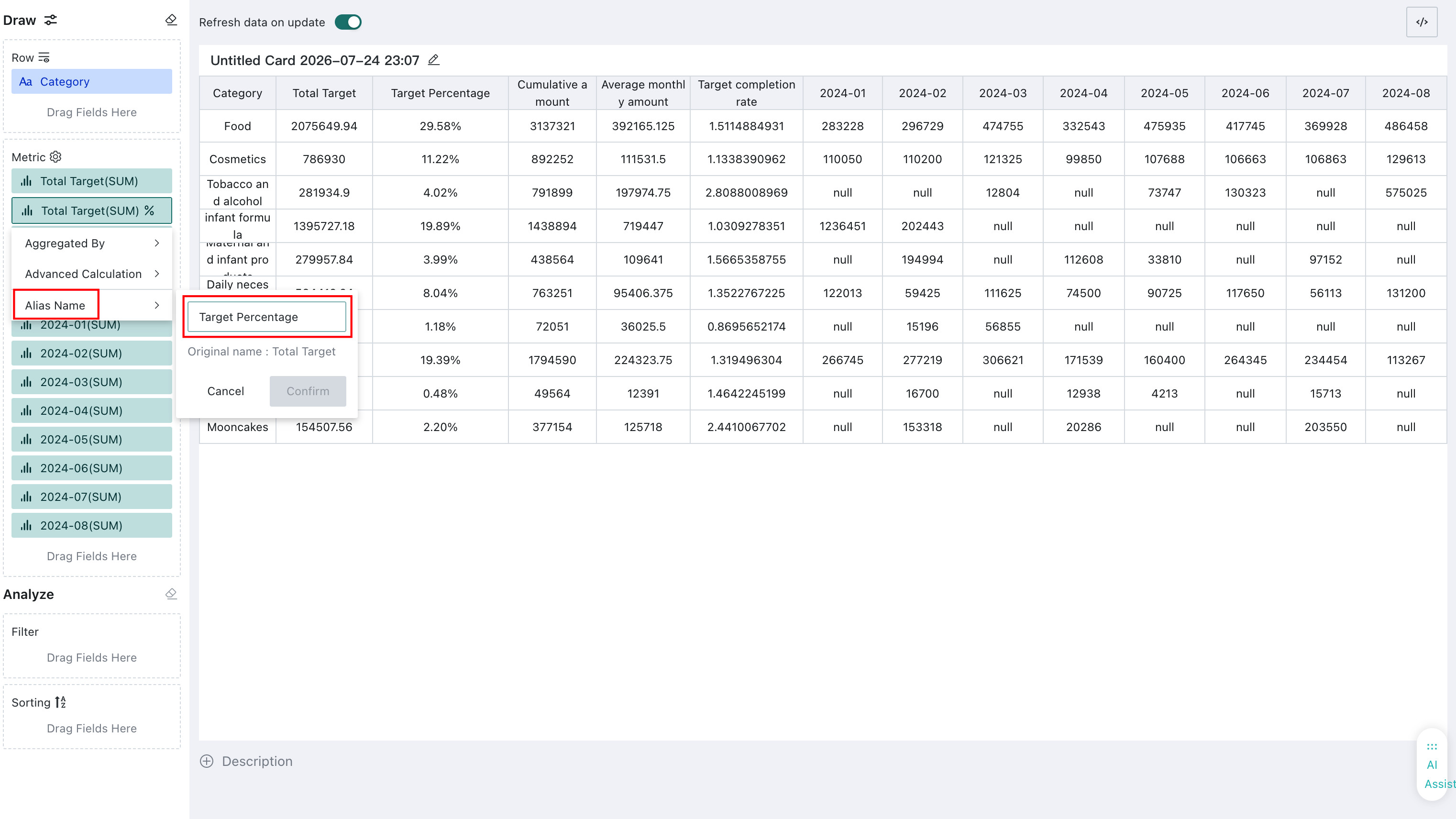
Target Totalinto the measure area again, click the field, and choose Advanced Calculation > Percentage of Total > By Column. To make the field easier to understand, rename it to Target Percentage.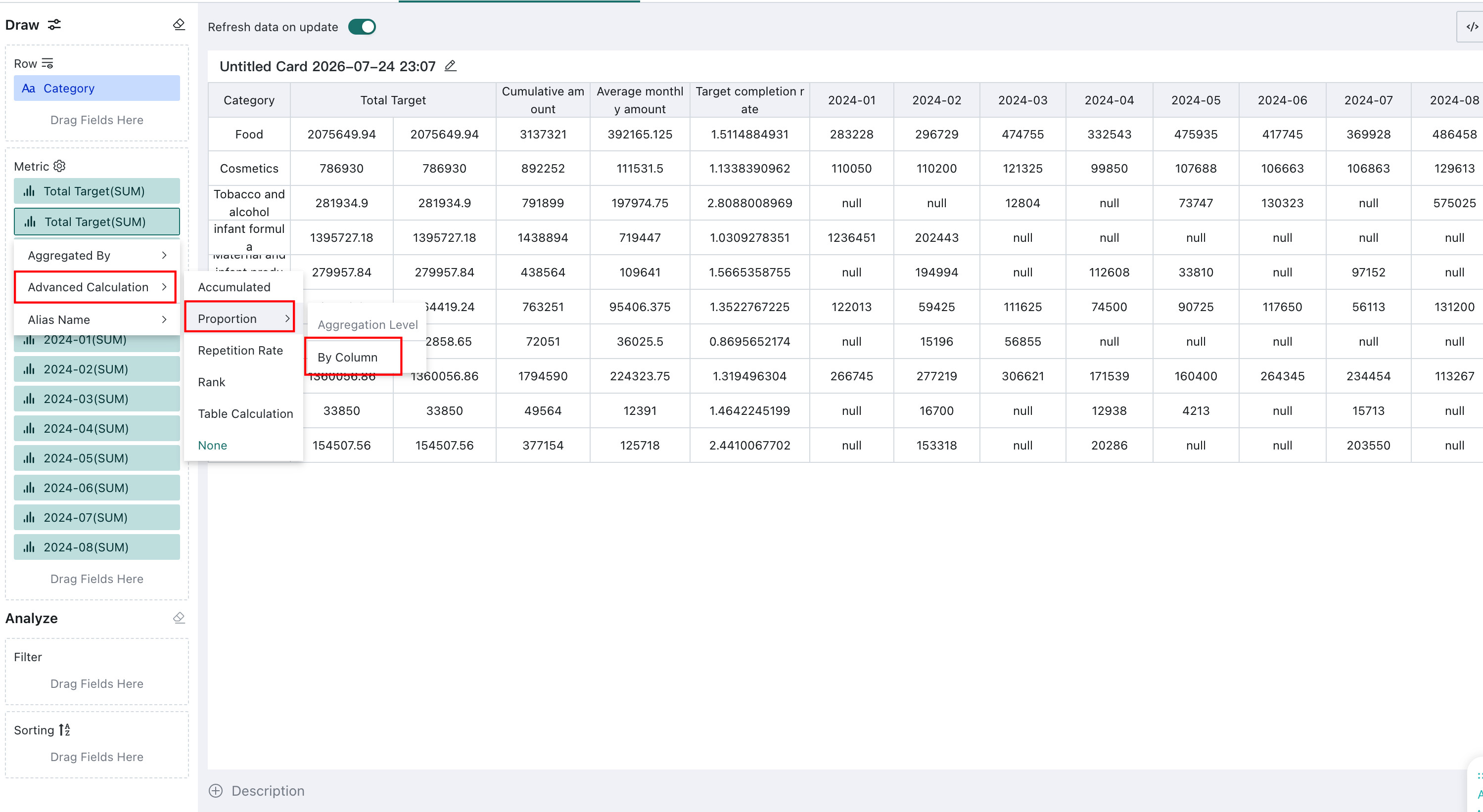
For details about percentage calculations in Advanced Calculation, see Advanced Calculation - Percentage of Total.
-
Configure the analysis area:
- Filters: none are required in this example
- Sort:
Category
-
After data preparation is complete, the result looks like the following image. After confirming the data is correct, click Save and Continue.
Template Editing
Configure the Static Header
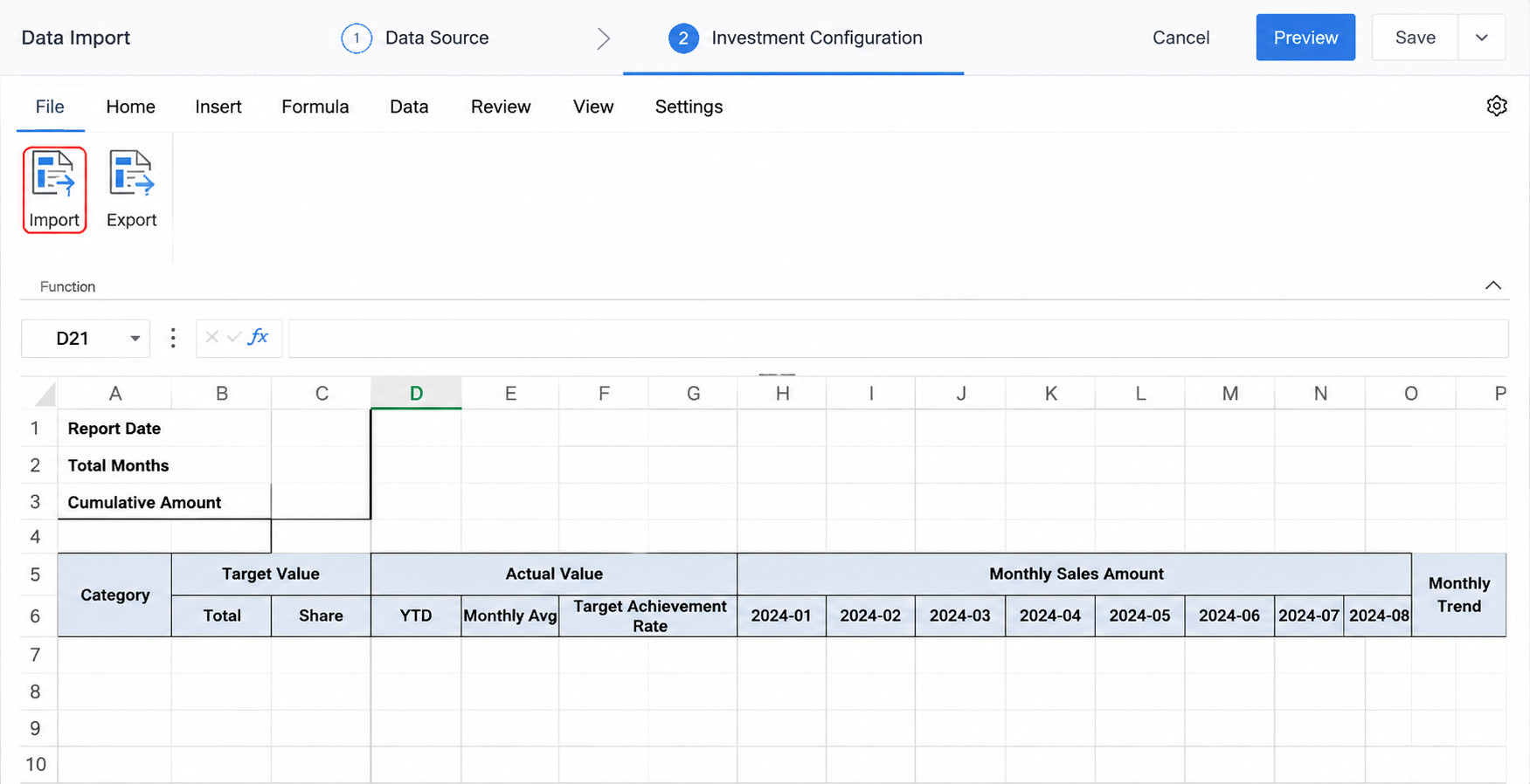
In this example, the static header is generated by importing a prepared Excel template: Practice Template. If no template is available in actual operation, you can also enter text manually in the corresponding positions to create the static header.
Click File > Import, select the template file, and open it.
Configure the Dynamic Header
-
Drag the dimension field
Categoryinto target cellA7, double-click it, and set its dynamic attribute to vertical expansion.NotesAfter a field from the view is dragged into a cell, it is automatically converted into a template cell and set to vertical expansion by default.
-
Click Preview for the report and confirm that the header expansion behaves as expected.
Configure Measure Fields
-
Drag the measure fields that need to be displayed into the worksheet template:
Drag fields such as
Target Total,Target Percentage, and the others one by one into cellsB7throughN7.NotesYou can hold
Shiftand select multiple fields, then drag them into the worksheet in batch and choose to paste them from left to right or from top to bottom.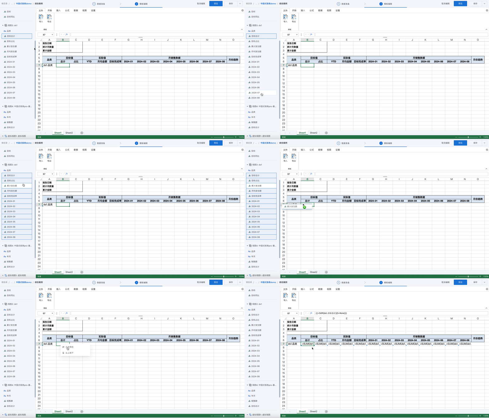
-
Configure a valid parent cell for each field:
In this example,
Target Total,Target Percentage,Cumulative Actual Amount,Average Monthly Actual Amount,Target Completion Rate, and the monthly fields from2024-01to2024-08all need to expand vertically by category. Double-click each corresponding field cell and set the parent cell toA7.NotesYou can select these cells in batch, right-click, and choose Batch Set Dynamic Attributes to configure the parent cell in one operation. In this case, the parent cells of
B7toN7can all be set toA7, as shown below.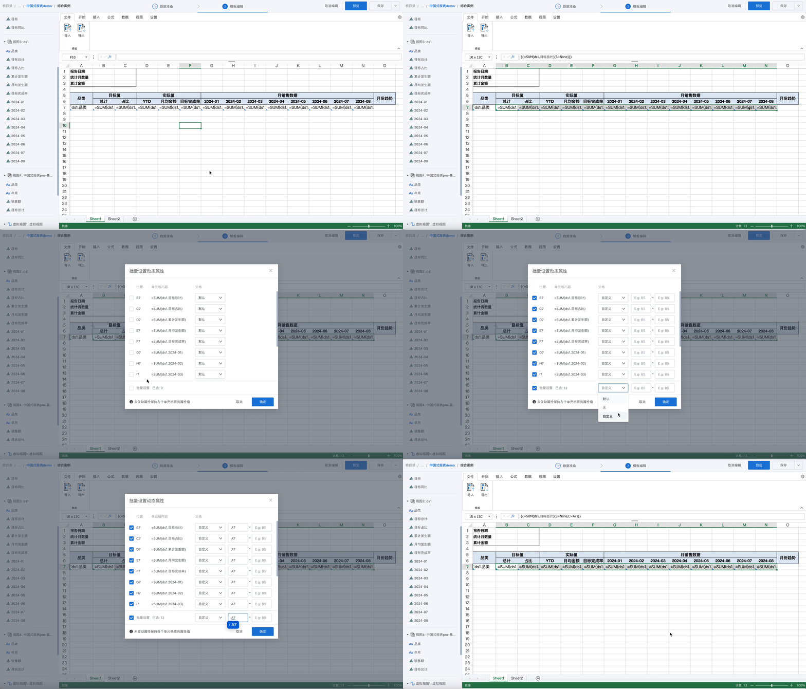 Notes
Notes- By default, the parent cell of a template cell is the nearest cell to the left plus the nearest cell above. For example, the default parent cell of
B7, whereTarget Totalis placed, isA7. - Empty cells, constants, and formulas beginning with
=cannot actively expand, so they cannot serve as valid parent cells for other cells. For example, the default parent cell ofC7isB7, but that is invalid, so its parent cell must be changed manually toA7.
- By default, the parent cell of a template cell is the nearest cell to the left plus the nearest cell above. For example, the default parent cell of
-
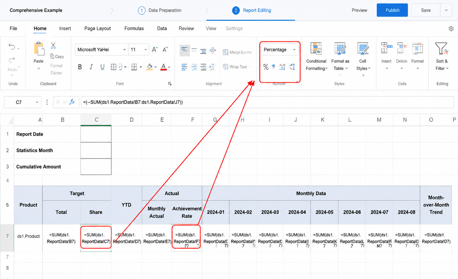
Beautify the data format:
Target PercentageandTarget Completion Rateshould use percentage formatting. Select cellsC7andF7, then configure them as percentages in the number settings and set the desired precision.
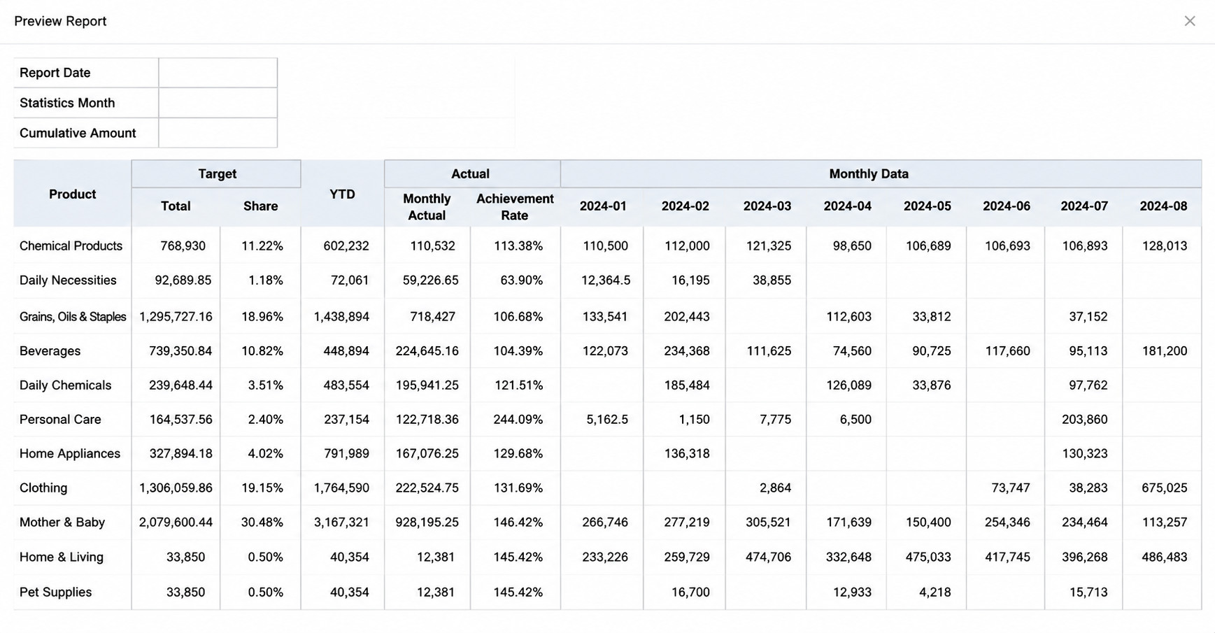
- Click Preview to see the current result.
Insert Sparklines
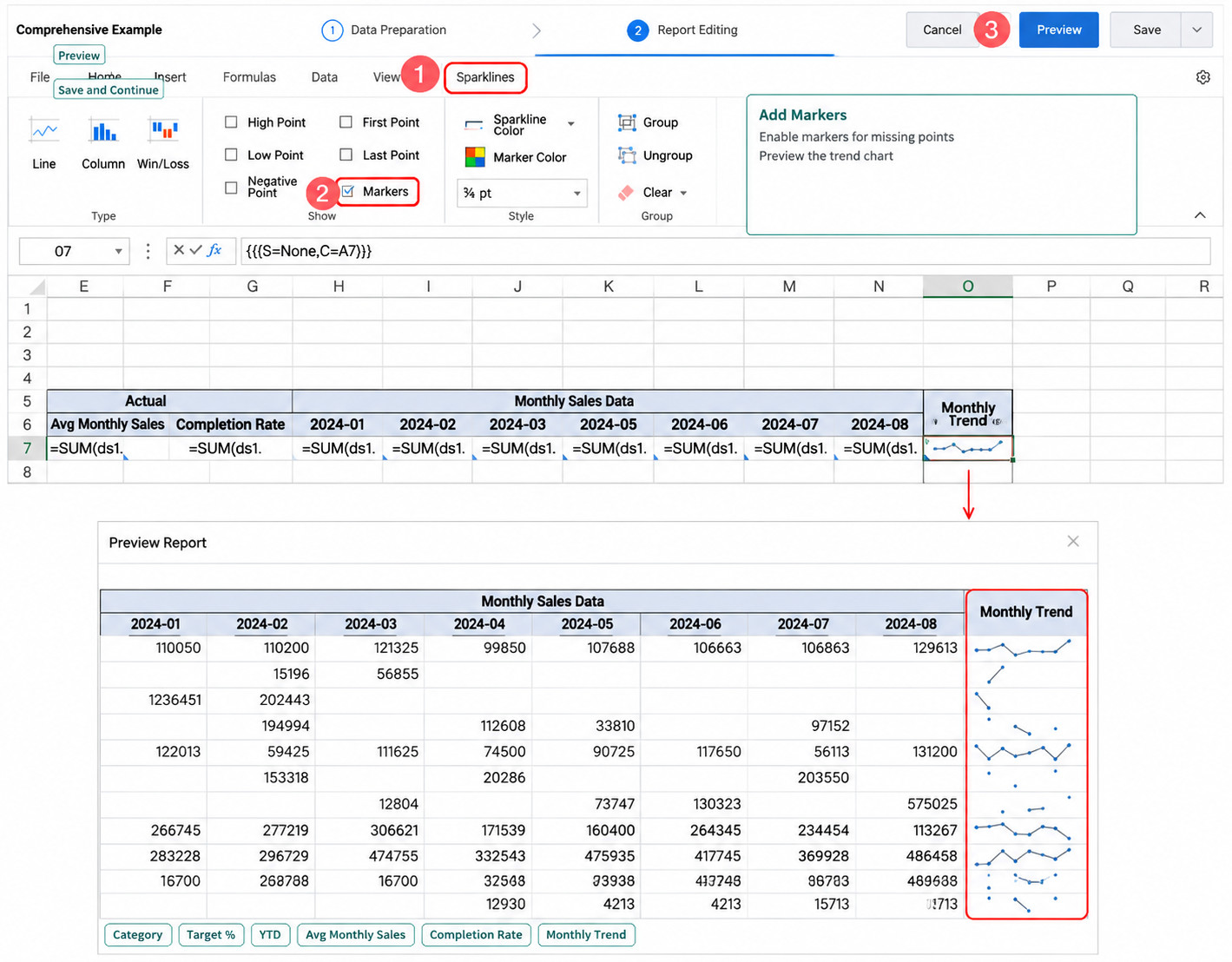
Under the Monthly Trend header, insert a trend chart for the monthly values from 2024-01 to 2024-08, and make it expand by category.
-
Select the range
G7:N7in batch, choose Insert > Sparklines > Line Sparkline, then configure the chart data range and the location where the sparkline should be placed.In this example, the chart should display data from
2024-01to2024-08, so the data range isG7:N7. Set the sparkline location toO7. It is recommended that you clear Formula Chart.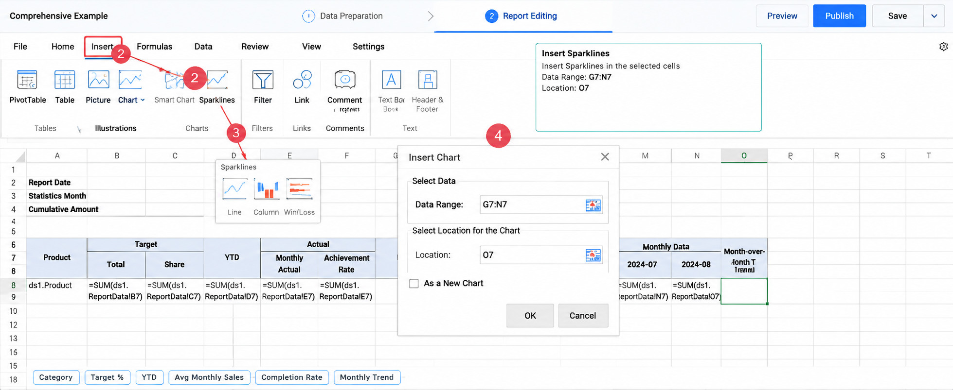
-
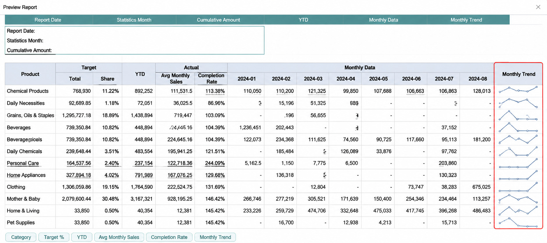
After the sparkline is inserted, only cell
O7contains the chart. Configure its parent cell so the monthly trend chart expands vertically by category:- Right-click
O7and choose Set as Template Cell. - Double-click
O7to open dynamic cell settings and set its parent cell toA7, so the monthly trend chart expands vertically byCategory. - Preview the result.
- Right-click
-
Some data points in the monthly trend chart may be missing. You can complete them by adding markers. After adding markers, preview the result again.
Use Functions to Get Target Values
-
Report Date should display the current date of the report day, using the function
TODAY().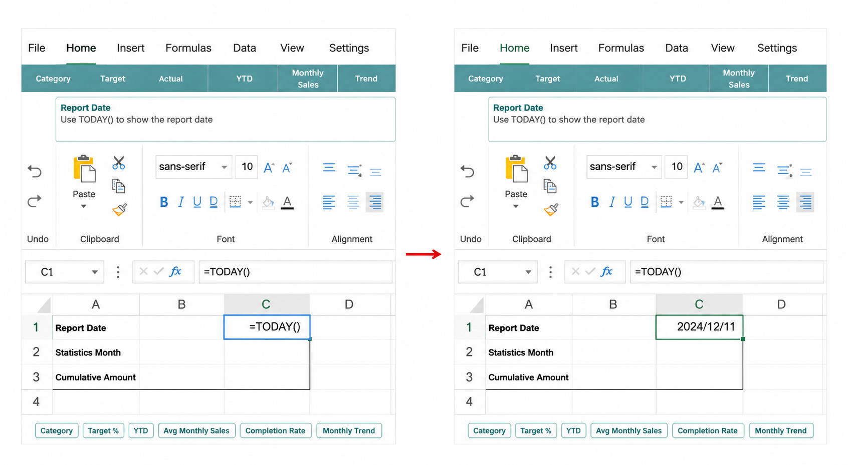
-
Number of Months should calculate the total number of month headers by counting the cells in
G6:N6, using the functionCOUNTA().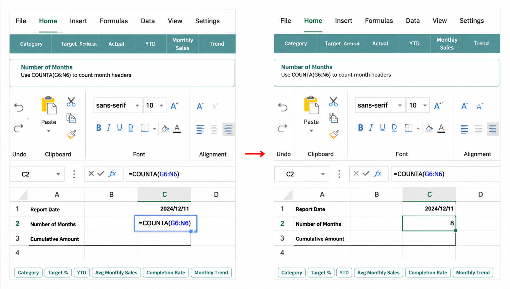
-
Cumulative Amount should calculate the total sales amount across all categories, that is, the sum of all vertically expanded
YTDvalues inD7, using the functionSUM().- Enter the formula
=SUM(D7). - Right-click and set
C3as a template cell.
NotesSince the function in
C3sumsD7, andD7is a dynamically expanding template cell, the result is incorrect unlessC3is also converted into a template cell.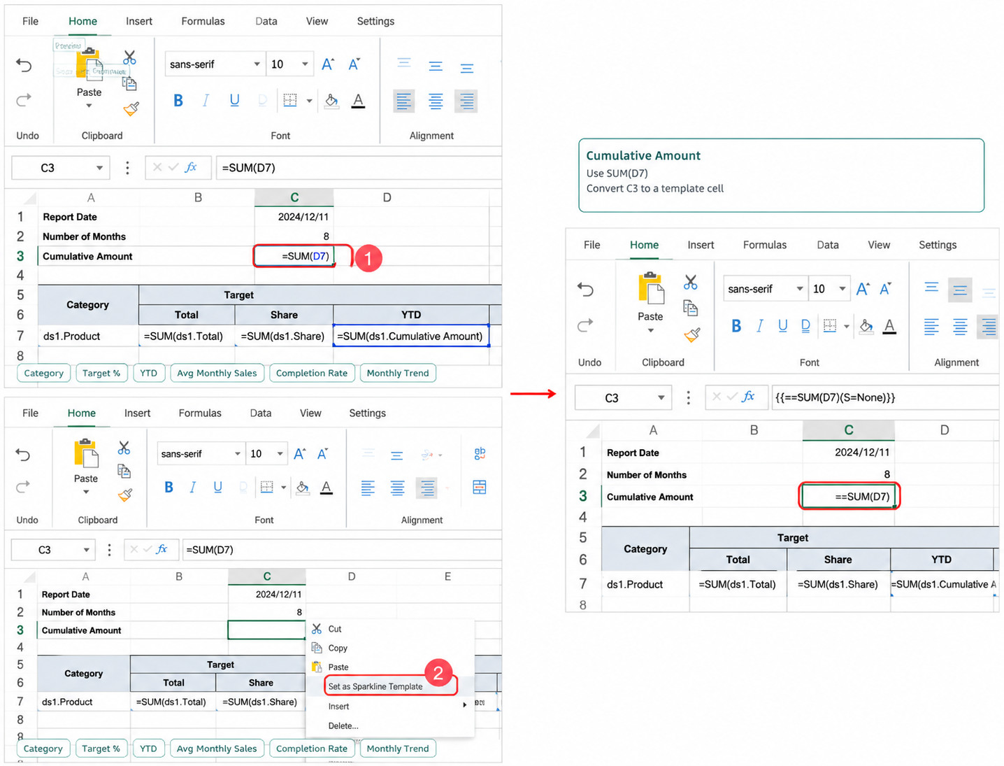
- Enter the formula
-
Preview the result.
Extended Example
This case produces the same configuration result as the one described above, but its data source uses a different data format: Chinese-style Reporting Pro - Basic Dataset 2.
Because of the different data format, the configuration steps also differ. See the video walkthrough for details: Chinese-style Reporting Pro - Basic Example Demo 2.